These notes on the basics around postgres internals are from the docs and also from Hironobu Suzuki’s Book on The Internals of PostgreSQL. The notes are intended to be brief, sometimes scant and many of the diagrams are taken from the book itself.
client app connects to the pg server so that a query can be transmitted
parser stage: query checked for syntax — forms a query tree
rewrite system: query tree + rules within rule bodies (rules stored in system catalogs) used to transform query
e.g. for realising views (i.e. virtual tables) – querying against a view makes the rewrite system transform it to access the base tables in the view definition instead
planner / executor: rewritten query tree to form a query plan — query plan will be passed to the executor
determines all the paths to the result, then determines the cheapest path. Cheapest path is expanded into a complete plan that the executor can use.
recursive execution by executor: steps through the plan tree to get the rows needed — uses storage system (scanning relations, doing sorting and joins…), evaluates qualifications. Returns rows.
lexing (via flex) and parsing (via bison) is done (they transform to the *.c forms using flex/bison ) and a parse tree is created
lexing: recognise identifiers, generating tokens that gets (see scan.l)
parser (see gram.y) has the grammar rules and actions to execute when rules are fired
this is structural, based on the syntactic structure of the given SQL
there’s no system catalog lookup for this, so the parse tree doesn’t have any semantic interpretations yet
this separation of raw parsing and semantic analysis is because semantic analysis involves system catalog lookups, which has to be within a transaction (for atomicity (?))
this is separation is fine because we can get control commands known from just doing structural analysis
helps with semantic meaning: which tables, functions, operators are referenced by the query
uses a query tree data-structure, which is similar in structure to the parse tree (from parser) but with differences in level of detail (that comes from doing semantic analysis)
sequential scanning of a table is the fallback default plan for a relation
we can do better if there’s an index defined on a relation.
conditions for using the index: the index will have keys (e.g. for b-trees) and operations within its operator class that we can use. If the query contains restrictions that match these, then the index can be used to explore a path.
scanning relations before finding paths for join relations; there’s multiple join strategies:
nested loop join:
right relation scanned once for every row found in the left relation — nested
easy to implement but time-consuming
merge join:
sort join attributes before joining so that scanning can be done in parallel — matching rows form join rows
sorting may be a separate explicit step or by scanning relation in a proper order using an index on the join key
hash join:
right relation scanned and loaded to hash table, with join attributes being hash keys — then the left relation is enumerated and the hash-table is used
since it’s a plan tree, we call the nodes plan node
they have the added ability to do selection (filtering on a boolean condition) and projection (derived column-set based on column values [scalar expressions])
planner must attach selection conditions from the WHERE clauses to the correct nodes of the plan tree
the plan-tree (from planner/optimizer) is recursively processed (by executor), in a demand-pull fashion.
this is referring to a pull-based model (dataflow terminology, the consumer demands and it affects when the node’s output is requested). Plan node is the source, the executor is the consumer.
Because work happens only on demand, LIMIT 10 really does stop after ten rows. The Seq Scan underneath may have read only a handful of pages. This is also why EXISTS subqueries and cursors behave well: you pay for what you consume.
Pipelining with low memory.
A row can flow from a scan through filters and joins to the client without ever being materialized in bulk. Memory use for those nodes is roughly one tuple at a time, not the size of the table.
Composability.
Every node speaks the same tiny interface, so the planner can stack arbitrary nodes in arbitrary shapes without the nodes knowing about each other.
Simple control flow.
Execution state lives in each node’s PlanState struct, so a node can be suspended between calls and resumed on the next pull. That’s what makes cursors (FETCH 10) natural.
limits:
some queries like sorting can’t be done lazily
complex queries are a matter of breaking down simple ones and just recursively doing them
the executor mechanism (see dispatch table here) works for the basic query typs (SELECT, INSERT, UPDATE, DELETE, MERGE)
for SELECT, the top-level executor needs to only send the rows returned by the query plan tree to the client
for the modifiers, there’s a ModifyTable top-level plan node (ref), they pass around TIDs (tuple-ids) to do their job
internally, tables and indices managed via their OIDs + physical data files managed by relfilenode, another id — typically relfilenode matches OID but not always
values may change on truncation, reindexing, clustering
8KB (8192B) fixed-length pages / blocks, 0-indexed, ids are called block numbers
internal layout depends on the type of data file
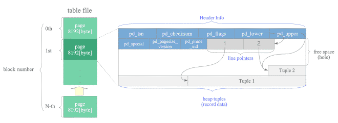
heap table file layout
Figure 1: heap table file layout diagram
it’s a “heap” because the tuples are stacked sequentially from the bottom of the page, KIV concurrency control and WAL to appreciate this part better
line pointers (4B) aka item pointer: point to the specific tuple in the record data (within the page); pointers form a simple array – reference using offset number
header data (24B), contains:
LSN of the xlog record with the most recent chagne to this page — 8B related to WAL
checksum
lower and upper line points: upper points to the beginning of the most recent heap tuple, lower points to the end of the line pointers — 2 different objectives to this!
special var for indexes (pointer to start of some special place specific to the index type (e.g. B-tree))
free-space / hole: the empty space between the end of the line pointers and beginning of the most recent tuple
identify specific tuple using TID (Tuple ID) = <block number of page that contains the tuple, offset number of the liner pointer>
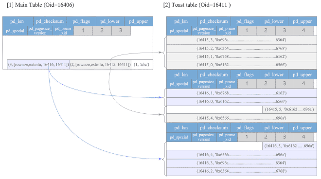
TOAST (the oversized-attribute storage technique)
there’s a threshold for tuples (TOAST_TUPLE_THRESHOLD ~ 2KB), when a tuple exceeds then it’s compressed
compression method is pglz
if size still exceeds even after compression, then uses a TOAST table (parent table stores pointer to TOAST table, where the actual data is stored)
Figure 2: relationship between the main table (tbl_toast) and the TOAST table (pg_toast_16406)
the data items within the toast table (tbl_toast) are limited to 10kb so TOAST pointers are kept using the varatt_external struct ( ref )
toast index is a composite of <chunk_id, chunk_seq>, retrieving TOASTed data will invoke an index-scan on the TOAST index to fetch the chunk_data segments in the right order
AI usage disclosureClaude Sonnet 5.5 · disambiguation
The outline of concurrency models relevant to db systems is ai-generated.
process model vs thread model:
Process model: each connection gets its own OS process with a private virtual address space. Anything shared must be set up explicitly (in Postgres: shared_buffers, lock tables, WAL buffers via shared memory, plus semaphores and signals). The MMU enforces isolation, so a wild pointer in one backend segfaults that backend and nothing else (the postmaster then restarts everything as a precaution, but that is a deliberate safety choice).
Thread model: many threads inside one process share one address space. Creation and context switches are cheaper, and sharing data is just dereferencing a pointer. The cost is that there is no memory-level isolation: one bad write or crash can take down the whole server, and all shared state needs careful synchronization.
What enables threads now:
Standardization: POSIX threads (IEEE 1003.1c) arrived in 1995, after Postgres’s design was set, and C11/C++11 later defined an actual memory model, so cross-platform threaded code has well-defined semantics.
Scalable OS support: Linux’s NPTL (mid-2000s) made 1:1 kernel threads cheap, backed by futexes for fast uncontended locking.
Ecosystem: thread-safe libc and libraries, plus tooling like ThreadSanitizer and Valgrind’s Helgrind for catching races.
The process model’s costs show up at scale: per-connection memory overhead, expensive connection setup (hence PgBouncer), and clunky dynamic shared memory, since processes may map the same segment at different addresses and so can’t share raw pointers. That’s why there is an ongoing community effort to move Postgres toward threads. It’s a huge refactor because so much code assumes process-global state is per-backend.
alternative concurrency models:
Event-driven / async (single-threaded loop on epoll/kqueue): nginx, Redis, Node.js. Great for I/O-bound work, but one slow handler blocks everyone.
Thread-per-core / shared-nothing: Seastar, ScyllaDB. One pinned thread per core owns its slice of data, with message passing between cores and no locks on the hot path.
M:N green threads / coroutines: Go goroutines, async/await runtimes (Rust Tokio). Many cheap user-space tasks multiplexed over a few OS threads.
Actor model: isolated entities with private state that communicate only by async messages (Erlang, Akka).
CSP: like actors, but communication goes through channels rather than addressed mailboxes (Go).
Pre-fork / process pool: Apache prefork, and Postgres is effectively this with a per-connection spawn.
Hybrids exist in databases too: MySQL is thread-per-connection, and Oracle uses processes on Unix but threads on Windows.
parent proc, does a bunch of init (e.g. shared memory area allocation, launching bg processes, starting replication-associated / bg-worker processes as needed)
backend processes
comms with client via single TCP connection, proc terminates on TCP disconnection
there’s no native connection pooling feature but frequent connecting / disconnecting is costly so it’s good to use connection pooling middleware (pgbouncer, pgpool-II)
background processes
for db management, there’s a bunch of reasons for having this — e.g. VACUUM and CHECKPOINT
some bg process examples:
bg writer: writing dirty pages from the shared buffer pool to persistent storage periodically
checkpointer: for checkpointing operations
autovacuum launcher :autovacuum-worker processes for VACUUM and ANALYZE – requests the postmaster to spawn these workers actually
WAL writer: changes to db blocks written to WAL summary files
statistics collector: likely deprecated, it’s now moved to the cumulative statistics system @ shared memory
logging collector
io worker: async read operations outsourced from backend processes
archiver: for log-archiving
replication-associated
for streaming and logical replication, KIV chapter 11 and 12; procs start when replication is configured and active (other than logical replication launcher that always starts by default)
types of replication-associated processes:
logical replication launcher: launch + manage apply worker processes for each subscription
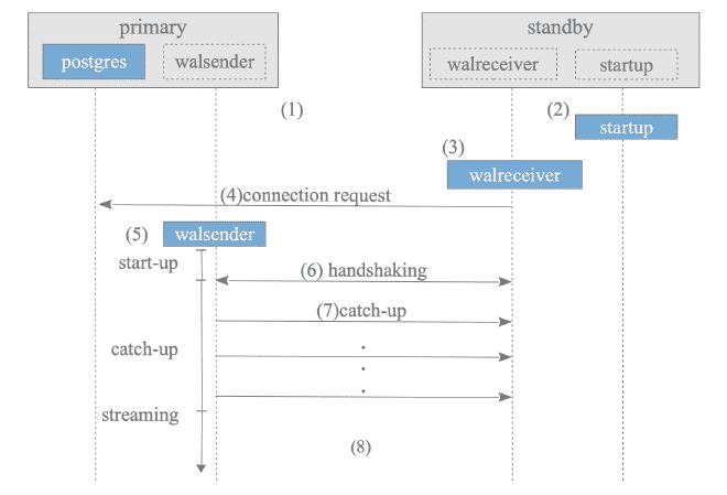
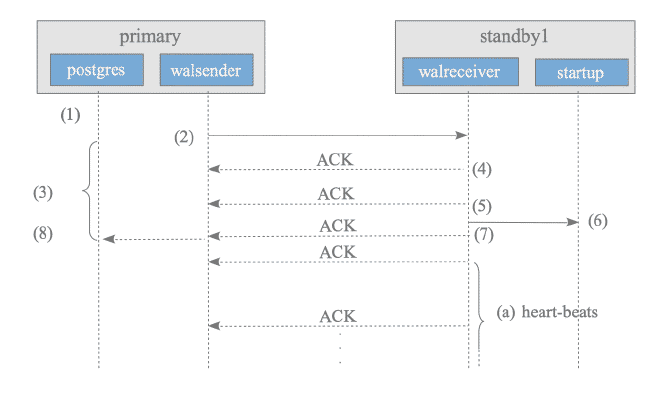
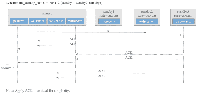
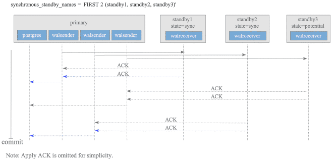
walsender: streaming replication (reads WAL data, sends to any of: connected standby server; logical replication subscriber; pg_basebackup client)
walreceiver: reception-side, for WAL data sent by primary server’s walsender
startup process: replyas WAL @ crash-recovery; for standby server in streaming replication, applies the received WAL data continuously
apply worker process: @ subscriber side of logical replication, gets decoded change messages from publisher’s walsender, applies to target tables
leader apply worker process: for parallel application (streaming = parallel); gets the streamed changes and dispatches to parallel apply workers
parallel apply worker process: launched by leader apply
background worker processes
to perform any user-implemented logic
comms via unix mechanisms (pipes, unix-domain sockets).
shared buffer pool: area used to load pages from tables / indexes from persistent storage so they can be operated on
this part is what the details from shared buffer readme was all about
WAL buffer: WAL data (aka XLOG records) has the transaction log; WAL buffer serves as temp storage area for WAL data before it’s flused to persistent storage
commit-log: CLOG holds state of all transactions for the CC (concurrency control) mechanisms
area for acms: managing semaphores and locks (LWlocks, shared, exclusive locks…)
area for background procs: coordination tasks by thigns liek checkpointer and autovacuum
area for transaction processing: maanging internal states, savepoints, 2PCs
there’s also dynamic shared memory (DSM) for supporting parallel queries
Both implement an equi-join by matching rows on a key. They differ in how they find the matches.
Hash join
Build phase: scan the smaller input and build an in-memory hash table keyed on the join column.
Probe phase: scan the larger input, hash each row’s key, and look up matches in the table.
No sort needed, no ordering produced. Cost is roughly linear in the sizes of the two inputs.
Equality only: hashing can’t answer < or > conditions.
Memory-sensitive: if the hash table exceeds work_mem, Postgres partitions both inputs into batches spilled to disk and joins batch by batch (a “Grace” style hash join, with a hybrid variant that keeps the first batch in memory).
Merge join
Requires both inputs sorted on the join key. Postgres either sorts them explicitly or gets sorted order for free from an index scan or an earlier sort.
Then it walks both sorted inputs in lockstep with two cursors, advancing whichever side is behind and emitting matches. Duplicate keys on both sides require backing up to rejoin the group.
Output is sorted on the key, which can help a later ORDER BY, GROUP BY, or another merge join.
Handles ordered comparisons better than hash, and can also do full outer joins.
Memory-light: the merge itself streams, and sorting spills to disk gracefully if needed.
When the planner picks which
Hash join usually wins on large, unsorted inputs with equality conditions, especially when one side fits in memory.
Merge join wins when inputs are already sorted (e.g. both have a B-tree index on the key), when sorted output is useful downstream, or when memory is tight.
Nested loop (the third strategy) wins when the outer side is tiny and the inner side has an index.
Intuition: hash join trades memory for skipping the sort, while merge join pays for sorting (or gets it free from an index) and then needs almost no memory to match. Both avoid the quadratic behavior of a naive nested loop.
subsystem encapsulated within a single backend, essentially the parts for “path of a query” above
planner and executor are highly complex, kiv future section
components:
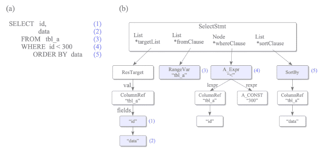
parser: for syntactic analysis
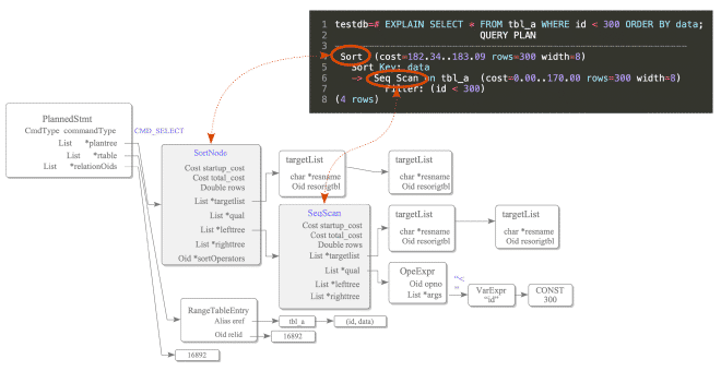
Figure 3: example of parse tree from a select statement
input: plaintext SQL
output: parse-tree for processing
it’s a 2-stage parse, isn’t really an example of “parse, don’t validate”
Partly. The “errors out on invalid syntax” half is right, but it isn’t really “parse, don’t validate” in Alexis King’s sense.
What’s accurate: the raw parser (gram.y, a Bison grammar plus a Flex lexer in scan.l) rejects anything that doesn’t match the grammar with a syntax error at or near .... And what it produces is a raw parse tree (RawStmt / SelectStmt nodes, etc.), not the original string, so downstream code never re-examines text.
Where the analogy breaks: “parse, don’t validate” is about parsing into a type that makes illegal states unrepresentable, so later code can’t receive bad input. Postgres splits the work in two stages, and the first one deliberately knows very little:
Raw parse (raw_parser): purely syntactic. It needs no catalog access, so it can’t know whether a table, column, function, or type exists. SELECT * FROM nonexistent parses fine.
Parse analysis (parse_analyze, the src/backend/parser/analyze.c and =parse_.c= files)*: semantic. It looks up names in the system catalogs, resolves types and operators, checks that columns exist, and so on, producing the Query tree. This is where relation "x" does not exist comes from.
The reason for the split is practical: transaction control statements like ROLLBACK must still be parseable and executable when the current transaction is aborted and catalog lookups would fail. So the raw parser stays catalog-free, and semantic checking is deferred.
The resulting Query tree is closer to the spirit of the idiom (a resolved, typed structure the planner can trust), but the tree node types are still general-purpose structs, and the planner/executor do assume invariants that the analyzer established rather than having them encoded in the type system.
A more accurate phrasing for your notes: “two-stage: a catalog-free raw parser that rejects invalid syntax and emits a raw parse tree, then parse analysis that does semantic checks against the catalogs and emits a Query tree.”
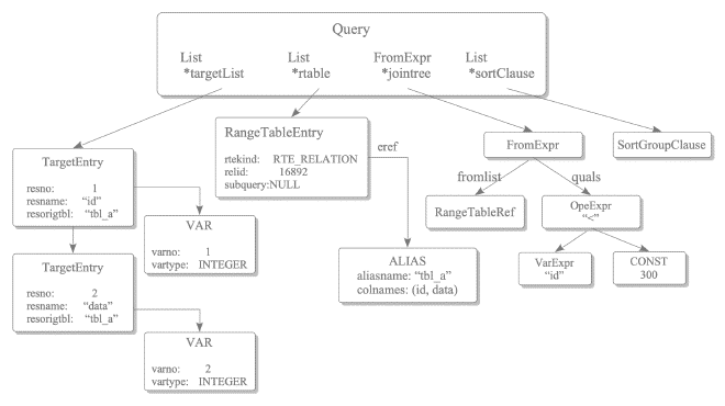
analyzer: for semantic analysis of parse tree
input: parse tree
output: query tree – ref docs here for components of the query tree
Figure 4: query tree of the select query
rewriter
input: query tree
output: query tree, with rules applied
planner
input: query tree
output: query-plan tree, optimised for efficient execution (cost-based optimsation)
query-rewrite rule system differs from stored procedures and triggers
example uses: query language procedures, views and versions
how they’re implemented :
(plain) views:
defined plain view is stored as a rule in pg_rules
so when it’s actually used, the rewriter will transform the range table node into a subquery parse tree given the view definition that is stored in the pg_rules system catalog
con: this makes it hard to make views updatable, there’s partial support for this, with some limitations
table-level filter predicates (e.g. id <= 8000) doesn’t reduce the range of pages scanned on disk; the filter is applied AFTER reading ALL tuples from the table
optimizer blanket-assumes that the pages must be read from storage: doesn’t consider whether the scanned pages are currently in the shared buffers or not.
estimation, regardless of the index method (B-tree, GIN, …) uses a common cost function (cost_index())
startup cost = cost for reading index pages to access the first tuple in the target table
run cost = sum of cpu and I/O costs fro both table and index
selectivity is an important component to run-cost calculation
is the estimated fraction of the index search range that satisfies the WHERE clause (a floating-point value between 0 and 1).
selectivity
refers to the selectivity of query predicates, estimated using either of the stats:
MCV (most common values)
for each column
there’s also a most common frequencies: list of frequencies for the values
histogram_bounds
what is it?
a histogram bound: A list of values that divide the column’s data into groups (buckets) of approximately equal population.
a histogram is a compressed summary of the value distribution, like a coarse CDF (cumulative distribution function). Because the buckets are equi-depth (each holds roughly the same number of rows), the bucket boundaries are essentially quantiles of the column. To estimate x < v, the planner:
counts the whole buckets entirely below v,
linearly interpolates within the bucket containing v,
divides by the number of buckets to get a fraction of rows.
Fine-grained where data is dense (boundaries bunch up), coarse where it’s sparse, which is why equal population rather than equal width matters.
Two things in your notes to tighten:
MCV vs histogram aren’t alternatives for the same case. Postgres uses them together. The MCV list covers the frequent values, and the histogram covers only the remaining non-MCV values. So histogram_bounds isn’t strictly “used when MCVs are unavailable”; it’s the fallback for values not in the MCV list, and for columns with no repeated values (unique-ish columns) it is the only one populated.
“Most common frequencies” is stored as most_common_freqs in pg_stats, and each frequency is a fraction of all rows, not a count.
If you want an analogy for your notes that is structurally closer, a B-tree’s internal nodes (separator keys partitioning a key range) are nearer to a skip list. The histogram is more like a quantile sketch or equi-depth partition summary.
values for the bounds represent the edges of the buckets
personal mental model: feels like something like a skip-list actually
Not really. The resemblance is superficial, and it’s worth correcting in your notes because the two structures do different jobs.
Where the intuition comes from: both let you “jump” over a lot of data using a coarse set of landmarks. A skip list has sparse upper levels that let you skip ahead; a histogram has sparse boundary values that tell you roughly where a value falls.
Why it breaks down:
Skip list
histogram_bounds
Purpose
Locate an element (a search structure)
Estimate how many rows match (a statistic)
Contains pointers to data
Yes, forward links
No, just values; it never points to rows
Used at execution time
Yes, to find data
No, only by the planner, before execution
Exact
Yes, finds the exact element
No, an approximation based on a sample
Maintained on every write
Yes
No, rebuilt by ANALYZE
A histogram never gets you to any data. It only lets the planner say “about N% of rows have =x < 500=”, which feeds the cost formula for choosing between a seq scan and an index scan.
A better mental model: a histogram is a compressed summary of the value distribution, like a coarse CDF (cumulative distribution function). Because the buckets are equi-depth (each holds roughly the same number of rows), the bucket boundaries are essentially quantiles of the column. To estimate x < v, the planner:
counts the whole buckets entirely below v,
linearly interpolates within the bucket containing v,
divides by the number of buckets to get a fraction of rows.
Fine-grained where data is dense (boundaries bunch up), coarse where it’s sparse, which is why equal population rather than equal width matters.
Two things in your notes to tighten:
MCV vs histogram aren’t alternatives for the same case. Postgres uses them together. The MCV list covers the frequent values, and the histogram covers only the remaining non-MCV values. So histogram_bounds isn’t strictly “used when MCVs are unavailable”; it’s the fallback for values not in the MCV list, and for columns with no repeated values (unique-ish columns) it is the only one populated.
“Most common frequencies” is stored as most_common_freqs in pg_stats, and each frequency is a fraction of all rows, not a count.
If you want an analogy for your notes that is structurally closer, a B-tree’s internal nodes (separator keys partitioning a key range) are nearer to a skip list. The histogram is more like a quantile sketch or equi-depth partition summary.
Suggested rewrite of that line: “histogram: equi-depth bucket boundaries (quantiles) over the non-MCV values; used only for selectivity estimation via interpolation, not for locating data.”
used when MCVs are unavailable (e.g. for unique, highly diverse integer / double types)
see the detailed explanations within the run cost section here
index correlations
statistical correlation between the physical row ordering and the logical ordering of the column values (range = [-1, +1])
total costs
values for some costs have to be tuned to make it more realistic
random_page_cost
e.g. note that the cost of random page I/O is excessively high (overestimate) compared to today’s SSD speeds for random access
selectivity estimation is actually challenging from the beginning of their invention
pg uses selectivity but broadly, db systems use cardinality
use the term “cardinality” henceforth
\[
Selectivity = \frac{Cardinality}{N_{tuple}}
\]
\(N_tuple\) is the total number of tuples (row) in the table
estimating cardinality is difficult
mainly because of relationships between different columns because they’re not necessarily independent, so correlation awareness matter here
there’s a good example of driving license given in the text here; the intuition is that just statistical approaches may not be good for such estimation because there may be other rules that should be encoded (e.g. drivers U18 can’t exist) and such dependencies that adds inaccuracies.
most RDMS planners calculate Cardinality by assuming that columns are mutually independent
this may be a huge source of inaccuracy for estimating costs
partial solution: extended statistics
capture correlations between columns by creating statistics objects
helps estimation results align more closely with the actual distribution, without independence assumptions
this can only be configured for columns within a single table, won’t apply to joins involving multiple tables, R&D still ongoing for cross-table cardinality estimation
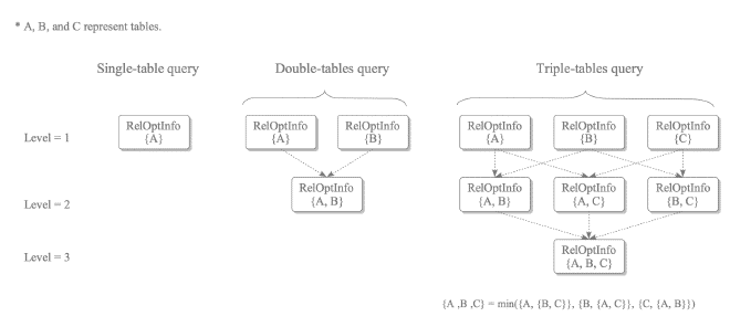
create a RelOptInfo structure (from within make_one_rel() (ref)); the RelOptInfo is stored within the simple_rel_array (ref)
estimate costs and add the access paths
sequential scan: path for sequential scan (worst, fallback)
index scan: if relevant indexes exist
bitmap scan: if a feasible
select cheapest path from all entries within pathlist of the RelOptInfo
estimate aux costs: for aux functions like LIMIT, ORDER BY, AGGREGATE
when there’s steps like sorting that happen, the way this is done is by creating a new RelOptInfo and creating a SortPath which links to the Path that is resolves from the non-sorted version of the query
for cases when there’s multiple paths, the final path is chosen by creating a new RelOptInfo and adding the cheapest paths from the other RelOptInfo s that have been created / found / exist. This step also gives an opportunity to prune trees.
Your understanding is half right. In Postgres, “relation” is broader than “table” but narrower than “any database object.”
Two senses of the word
Theoretical (relational model): a relation is a set of tuples, which is what SQL’s tables, subquery results, and join outputs all model.
Postgres catalog sense: a relation is anything stored in pg_class, the catalog table with one row per relation. This is what relation "x" does not exist refers to, and what Relation structs (RelationData) and RangeVar refer to in the source.
What counts as a relation (pg_class.relkind)
ordinary table (r)
index (i)
sequence (S)
view (v)
materialized view (m)
composite type (c)
TOAST table (t)
foreign table (f)
partitioned table (p) and partitioned index (I)
The common thread is that each has a row in pg_class and a relfilenode (for the ones with storage), meaning files on disk. Views and composite types are in pg_class but have no storage.
What is not a relation: functions (pg_proc), types (pg_type), operators (pg_operator), roles, schemas, extensions, triggers, constraints. These live in their own catalogs. So “any db object” overshoots. It’s more “any object that behaves like a named row-set or has relation-like storage.”
Meaning in your planner notes
Here “relation” means something narrower still: a thing that can appear in a FROM clause and be scanned, i.e. a range table entry (RangeTblEntry) in the query tree. That includes:
base relations (real tables, RTE_RELATION)
subqueries (RTE_SUBQUERY)
function calls returning sets (RTE_FUNCTION)
VALUES lists, CTEs, and join results
This is why the planner structure is called RelOptInfo (“relation optimization info”): it holds the paths and cost estimates for any scannable row-set, whether a base table or an intermediate join result. For your single-table case there’s exactly one base RelOptInfo in simple_rel_array, indexed by range table index. In multi-table queries, join planning builds additional =RelOptInfo=s for join relations, with each joinrel being “the result of joining this subset of base relations.”
Indexes are relations in pg_class, but they aren’t entries in simple_rel_array as scan targets. They’re attached to their table’s RelOptInfo via its indexlist as =IndexOptInfo=s, which is how the planner generates index paths for that table.
Suggested note:“relation (pg sense): anything with a pg_class entry (tables, indexes, sequences, views, matviews, …). In the planner, RelOptInfo is a narrower notion: any scannable row-set in FROM (base table, subquery, join result) that carries candidate paths and costs.”
(1) ExecConstraints() checks NOT NULL constraints and CHECK constraints.
Block 2: Insert the heap tuple
(2) table_tuple_insert() inserts the tuple into the heap table.
Block 3: Insert index tuples and enforce uniqueness
(3) ExecInsertIndexTuples() processes all indexes belonging to the table.
(4) index_insert() inserts the corresponding index tuple into each index.
(5) _bt_check_unique() checks whether a conflicting key already exists. UNIQUE and PRIMARY KEY constraints are enforced here.
loaded from pg catalog (pg_constraint) into memory and the corresponding expression (for check constraints) are evaluated for each inserted / updated tuple
same for UPDATE statements
PRIMARY KEY and UNIQUE
check index in \(O(log n)\) time when possible
FOREIGN_KEY constraints
since it involves other tables, implementation is more complex
the referenced row in the other table may be locked by the original statement using a FOR KEY SHARE
during the duration of the FK constraint check
select statement executed via the SPI (server programming interface)
so we can have cases where a single tuple into the child table executes an additional internal SELECT query
direct FOREIGN KEY validation, a new execution path
instead of the internal SELECT query, validate the FOREIGN KEY directly by probing the referenced index if a suitable index backs the referenced PRIMARY KEY or UNIQUE constraint
it’s an optimisation because it avoids the SPI-query-execution-path
avoids the planner, executor, SPI overheads that would have had if it was an internal SQL statement that was getting evaluated
all the SQL standard join operations are supported by PG ( INNER JOIN, LEFT/RIGHT OUTER JOIN, FULL OUTER JOIN )
operations are implemented via a bunch of join algorithms:
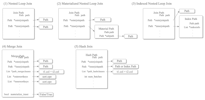
nested loop join – multiple variations
merge join – multiple variations
hash join
difficulty of cardinality estimation for multiple-table joins
estimation relies on the assumption that columns across tables are statistically independent, but this assumption gets weaker across multiple join tables — this is a significant limitaiton
has no startup cost, run cost = \(O(N_{outer} * N_{inner})\) becaues the operation is kind of like a cross-product
the other, specific nested loop join algos are used actually
materialized nested loop join
insight: the join is based off the inner table, so we can materialise it and reuse it
Materialization allows for more efficient processing of inner table tuples compared to relying on the buffer manager
how to materialize? abstracted by temporary tuple storage module, see here
depends on the total size of the tuples being stored:
small enough to use work_mem
larger; need to use temp files
materialize:
has no startup operation — no startup cost
eventually when the nested looping is done, this materialized view is rescanned so remember to include the rescanning costs
indexed nested loop join
if the inner table already has an index already then that can be used instead of running a whole sequential scan on it
if the planner uses that, then it’s indexed nested loop join
scans the outer table only once (despite its naming)
consider this example :
EXPLAINSELECT*FROMtbl_cASc,tbl_bASbWHEREc.id=b.id;/*
QUERY PLAN
--------------------------------------------------------------------------------
Nested Loop (cost=0.29..1935.50 rows=5000 width=16)
-> Seq Scan on tbl_b b (cost=0.00..73.00 rows=5000 width=8)
-> Index Scan using tbl_c_pkey on tbl_c c (cost=0.29..0.36 rows=1 width=8)
Index Cond: (id = b.id)
(4 rows)
*/
Code Snippet 2:
query plan for an indexed nested loop join
the cost of accessing the inner table is the cost of looking up the inner table for a tuple that satisfies the index condition (i.e. i = b.id)
this path is called the parameterized (index path) (see optimizer readme)
how it works is that whenever a tuple is received from the outer table via a sequential scan, the index scan path identifies the corresponding inner tuples to be joined.
other variations
the idea is that if an index attribute can serve as an access predicate in the WHERE clause, the search range of the outer table is narrowed. This can drastically reduce the cost of the nested loop join
variations:
nested loop join with outer index scan
materialized nested loop join with outer index scan
merge joins are for natural joins and equi-joins (equality condition for joining)
on natural joins: natural join = equi-join on all same-named columns, deduplicated in output; a special case of equi-join, so merge/hash join can implement it. Prefer explicit ON/USING.
there’s an initial and final cost function and the estimation for the merge join uses them
variation: merge join
sorting for the merge join: once again, whether working memory or temp files depends on the number of tuples
example:
EXPLAINSELECT*FROMtbl_aASa,tbl_bASbWHEREa.id=b.idANDb.id<1000;/*
QUERY PLAN
-------------------------------------------------------------------------
Merge Join (cost=944.71..984.71 rows=1000 width=16)
Merge Cond: (a.id = b.id)
-> Sort (cost=809.39..834.39 rows=10000 width=8)
Sort Key: a.id
-> Seq Scan on tbl_a a (cost=0.00..145.00 rows=10000 width=8)
-> Sort (cost=135.33..137.83 rows=1000 width=8)
Sort Key: b.id
-> Seq Scan on tbl_b b (cost=0.00..85.50 rows=1000 width=8)
Filter: (id < 1000)
(9 rows)
*/
variation: materialized merge join
the inner table is materialized to make the inner table scans more efficient
so, there’s a Materialized node for the query plan
SETenable_hashjoinTOoff;SETenable_nestloopTOoff;EXPLAINSELECT*FROMtbl_cASc,tbl_bASbWHEREc.id=b.idANDb.id<1000;/*
QUERY PLAN
--------------------------------------------------------------------------------------
Merge Join (cost=135.61..322.11 rows=1000 width=16)
Merge Cond: (c.id = b.id)
-> Index Scan using tbl_c_pkey on tbl_c c (cost=0.29..318.29 rows=10000 width=8)
-> Sort (cost=135.33..137.83 rows=1000 width=8)
Sort Key: b.id
-> Seq Scan on tbl_b b (cost=0.00..85.50 rows=1000 width=8)
Filter: (id < 1000)
(7 rows)
*/
NOTE: the inner /outer table is chosen based on cost estimations and not by the FROM-clause order.
Your revised reading is right: the order of tables in the query text does not determine inner vs outer. The planner chooses, based on cost.
What decides it
For each join, the planner considers both orderings (A outer / B inner, and B outer / A inner) and adds a path for each to the join rel via add_path(). The cheaper one wins. FROM tbl_c, tbl_b is just a set of relations to join, and the planner is free to reorder it. The textual order of the FROM list and of the a.id = b.id condition doesn’t matter (equality is symmetric, and the planner normalizes it).
Reading the plan
In EXPLAIN output, the first child under a join node is the outer (left) input and the second child is the inner (right) input. That is the only reliable way to tell. In your examples:
Example 1: outer = tbl_a, inner = tbl_b
Example 2: outer = tbl_x, inner = tbl_y (the one wrapped in Materialize)
One correction to your framing: outer is the first/top child, which is conventionally the “left” input, not the right. So your original guess had the sides reversed, and the textual order of the query doesn’t map onto either.
Why the planner picks as it does in your examples
Example 3:tbl_c has a primary key index on id, so an index scan hands back rows already sorted on the merge key, with no Sort node needed. That path’s pathkeys match the merge condition, which is what makes it cheap. tbl_b is filtered (id < 1000) down to about 1000 rows, so sorting it is cheap. Cost-wise this beats sorting all 10000 rows of tbl_c.
Example 2: the Materialize goes on the inner side because a merge join may need to rescan/back up over the inner input when there are duplicate keys, and a Sort node’s output isn’t cheaply rescannable in general. Materializing makes those rewinds cheap. Note this is a cost decision too: it appears when the planner estimates the rescan cost outweighs the materialization cost.
Nuance for merge join specifically: unlike nested loop, where the outer/inner choice matters a lot (outer is scanned once, inner once per outer row), merge join is nearly symmetric, since both sides are scanned once in lockstep. The difference comes from the inner side’s possible backing up and from which side is already sorted. So the choice is subtler, driven by sort costs and rescan behavior.
On the name “merge join with outer index scan”: it just means the outer input is an index scan, which matches what you saw.
Suggested note:“Outer/inner is chosen by the planner by cost, not by FROM-clause order. In EXPLAIN, first child = outer, second = inner. Both orderings are costed and compete in the join rel’s pathlist. An index scan on the join key can supply pre-sorted input, avoiding a Sort.”
uses index scan within a hash join whenever possible
example:
EXPLAINSELECT*FROMpgbench_accountsASa,pgbench_branchesASbWHEREa.bid=b.bidANDa.aidBETWEEN100AND1000;/*
QUERY PLAN
------------------------------------------------------------------------------------------------------
Hash Join (cost=1.88..51.93 rows=865 width=461)
Hash Cond: (a.bid = b.bid)
-> Index Scan using pgbench_accounts_pkey on pgbench_accounts a (cost=0.43..47.73 rows=865 width=97)
Index Cond: ((aid >= 100) AND (aid <= 1000))
-> Hash (cost=1.20..1.20 rows=20 width=364)
-> Seq Scan on pgbench_branches b (cost=0.00..1.20 rows=20 width=364)
(6 rows)
*/
during probe phase, executor identifies and retrieves the required tuples from pgbench_accounts using an index_scan
doing this in the probe phase restricts the number of outer table tuples that need to be probed against the hash table — that’s why there’s a performance improvement
it’s about combining individual table access paths with joins to build a plan tree for the entire query — that’s how it extends from single-table queries
the ordering matters: join orders, join methods and how it handles the large search space when query contains many tables
method for transmitting the deparsed SQL statements is fdw-extension-dependent — there has to be a conversion feature implemented by the extension to allow compatibility
postgres_fdw is more complex, has xact management and cursors
default remote transaction isolation level is REPEATABLE READ — ref reason in official docs here
it has push-down capabilities (delegation) for things like aggregations
LIMITATION: pg’s fdw doesn’t detect deadlocks; there’s no support for distributed lock mangement and distributed deadlock detection — so cross-server deadlocks can occur
an example of a deadlock condition that is not detected and remains stalled indefinitely:
Client A updates a local table tbl_local followed by a foreign table tbl_remote, while Client B updates tbl_remote followed by tbl_local in the opposite order.
variant used by MVCC is SI (Snapshot Isolation) – this is REAPEATABLE READ isolation level in pg
Table 1:
comparing isolation levels in PG
Level
Snapshot
Dirty read
Non-repeatable
Phantom
Write skew / RO anomaly
READ COMMITTED (default)
per statement
no
possible
possible
possible
REPEATABLE READ (SI)
per transaction
no
no
no
possible
SERIALIZABLE (SSI)
per transaction + tracking
no
no
no
no
the pg default isolation level is READ COMMITTED: snapshot per statement
SI implementation:
others, like Oracle, use rollback segments
PG implementation is simpler:
new data item is directly inserted into the relevant table page,
when reading, pg selects the appropriate version of an item by applying visibility check rules. The xmin/xmax Visibility checking mechanisms are for this.
SI prevents the following anomalies in the ANSI sql standard:
Dirty reads
Non-repeatable Reads
Phantom reads
prevents lost updates via first-updater-wins: so concurrent updates abort
SI can’t achieve true serializability because of serialization anomalies (not captured by the SQL standard):
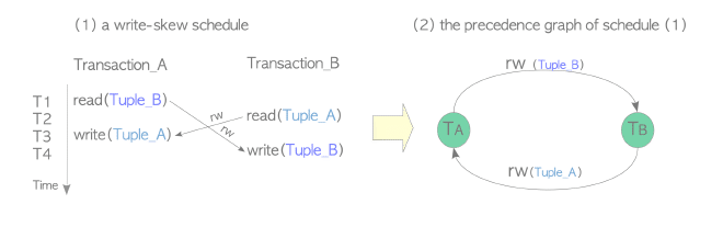
Write skew
2 xacts each reading an overlapping set of rows, and making a disjoint write each based on what they read and both commit — they don’t encounter write conflicts @ the row level so first-updater-wins doesn’t trigger and abort but the combined result violates an invariant that a serial order wouldn’t have done.
Classic example: two doctors both going off-call after each checking that the other is still on-call.
Read-only transaction Skew
a read-only transaction can observe a state that is inconsistent with any serial order, even though the read-only transaction itself writes nothing. It requires a third transaction, so it’s subtler than plain write skew.
SSI (Serializable Snapshot Isolation) implementation adds the ability to do serialization detection and resolving of conflicts, if any.
key idea: in an SI history, any non-serializable execution contains a cycle in the dependency graph with two adjacent rw-antidependencies (T1 →rw T2 →rw T3, where T1 reads something T2 later overwrites, and so on) forming a “dangerous structure.”
how does it work? tracking of rw-conflicts using SIREAD locks (predicate locks)
may have false positives
S2PL ( strict 2-phase locking )
needs to block readers when a writer writes an item because the writer acquires an exclusive lock for the item
identification, used in things like determining visibility of tuples
for the visibility purposes, txids are for tuple-stamping
txids assigned lazily: at the first write (or on explicit txid_current()), not at transaction start. Read-only xacts only have a vxid (backend_id / local_xid). Some special ids:
0: invalid
1: bootstrap txid, used @ cluster init
2: frozen txid
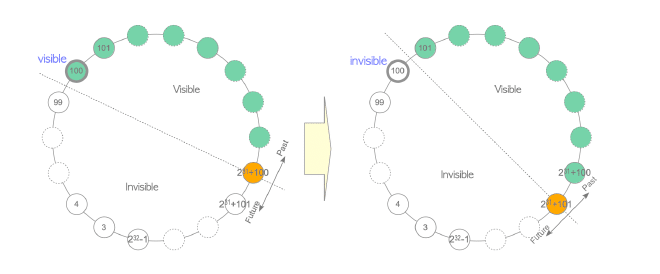
there’s an ordering to the ids and so they’re comparable — greater id number is in the future
the id-space is circular — so there may be cases of txid wraparounds being a problem
xact manager will provide a snapshot to a backend process when requested, specific to that point in time
timing depends on the xact’s isolation level:
if under READ COMMITTED, then xact obtains a new snapshot whenever sql command is exec-ed
if under REPEATABLE READ, SERIALIZED isolation levels then obtains a snapshot only when first SQL command is executed
snapshots needed for visibility check of tuples
when doing a visibility check, active xacts in the snapshots must be treated as inprogress even if they’re already in a final state (committed / aborted)
see detailed example here with 3 sequential transactions
so we get 10 selected rules for our basic understanding here, it’s based on the status of t_xmin
t_xmin is ABORTED
always invisible because the xact that inserted the tuple failed (RULE 1)
t_xmin is IN_PROGRESS
generally invisible (rules 3 and 4)
RULE 3: tuple has been deleted / updated by the current xact: if t_xmin = current_txid and t_xmax is valid
RULE 4: tuple inserted by another transaction and its status is IN_PROGRESS : if t_xmin != current_txid
means that uncommitted changes from one xact are invisible to other xacts
visible under rule 2 for inserting transaction (exception)
RULE 2: when t_xmin = current_txid and t_xmax = INVALID (then it’s an insertion)
tuple is visible to the current xact itself
t_xmin is COMMITTED
is generally visible (Rules 6, 8, 9)
RULE 6: inserted, committed and never deleted / updated before / aborted then it’s ‘visible’
RULE 8: if t_xmax is IN_PROGRESS and t_xmax != current_txid
means deleting xact is still in progress and not finalised yet (committed / aborted)
so it’s visible
RULE 9: t_xmax is active in the snapshot then the deleting xact is being treated as in-progress so the tuple is visible
has 3 exceptions
RULE 5: invisible if the inserting xact is still in progress
have to treat tuple as invisible if t_xmin is treated as in-progress
if in the obtained snapshot, the t_xmin is ‘active’ then it’s invisible
RULE 7: tuple is logically deleted / updated: if t_xmax = current_txid (i.e. current xact has deleted / updated it) so it should be invisible
RULE 10: tuple is logically deleted / updated: if t_xmax is NOT active in the obtained xact snapshot, means another xact has committed its deletion / update and so the tuple is invisible
AI usage disclosureClaude Sonnet 5.5 · codebase mapping
This section is ai-generated.
The code for these rules is mostly in one file: src/backend/access/heap/heapam_visibility.c. Before PG 12 it was src/backend/utils/time/tqual.c, which is what older blog posts and mailing-list threads refer to.
Where to start
HeapTupleSatisfiesMVCC() is the function that implements the rules you pasted. It’s the one used for ordinary snapshots (READ COMMITTED, REPEATABLE READ and SERIALIZABLE queries).
XidInMVCCSnapshot() in the same file is the “=Snapshot(t_xid) = active=” test.
HeapTupleSatisfiesVisibility() is the dispatcher. It switches on snapshot->snapshot_type, so you can see the other visibility semantics alongside MVCC: SNAPSHOT_SELF, SNAPSHOT_ANY, SNAPSHOT_DIRTY, SNAPSHOT_TOAST, SNAPSHOT_HISTORIC_MVCC (logical decoding) and SNAPSHOT_NON_VACUUMABLE.
HeapTupleSatisfiesVacuum() and HeapTupleSatisfiesUpdate() answer different questions (“can VACUUM remove this?” and “can I update this?”), and comparing them with the MVCC one is instructive.
Supporting pieces
src/include/access/htup_details.h has the tuple header layout (t_xmin, t_xmax, t_cid, t_infomask) and the HEAP_XMIN_COMMITTED, HEAP_XMIN_INVALID, HEAP_XMAX_COMMITTED etc. bit definitions.
src/include/utils/snapshot.h has the SnapshotData struct (xmin, xmax, xip[], subxip[], curcid).
src/backend/storage/ipc/procarray.c has GetSnapshotData(), which builds the snapshot by scanning running backends.
src/backend/access/transam/transam.c has TransactionIdDidCommit() / TransactionIdDidAbort(), which consult clog (access/transam/clog.c).
src/backend/access/heap/README.tuplock covers the locking-related xmax semantics.
How the code differs from the book’s rules
The code is not a table of rules. It’s an imperative decision tree, and a few design choices only show up when you read it:
Hint bits come first. The function checks t_infomask before touching clog. If HEAP_XMIN_COMMITTED is already set, the commit-status lookup is skipped entirely. When it does have to look up a status, it writes the result back with SetHintBits(). The book’s “Status(t_xmin) = COMMITTED” is conceptually a clog lookup, but in practice it’s mostly a bit test.
The snapshot check comes before the clog check. For an xid that isn’t the current transaction, the code calls XidInMVCCSnapshot() first and only then TransactionIdDidCommit(). If the xid is in the snapshot (in progress, or in the future, as far as this snapshot is concerned), the tuple is treated as not committed, regardless of what clog says now. This is why the book’s Rules 5 and 9 exist as special cases. Order matters here for race-condition reasons, which the comments explain.
XidInMVCCSnapshot() is cheap in common cases. It compares against snapshot->xmin (anything older is definitely not active) and snapshot->xmax (anything at or beyond is definitely “in the future”), and only searches the xip array for xids in between. There’s also separate handling for subtransactions via subxip and suboverflowed.
“Current transaction” is more than one txid.TransactionIdIsCurrentTransactionId() covers subtransactions, and the command id (cmin=/=cmax vs snapshot->curcid) decides whether a change made earlier in the same transaction is visible to the current statement. The book’s Rules 3 and 7 are the simplified version of this.
Cases the book’s table omits.xmax may be a multixact (HEAP_XMAX_IS_MULTI, used for shared row locks) or merely a locker (HEAP_XMAX_LOCK_ONLY), in which case the tuple is not deleted at all. A good chunk of the function’s length is handling these.
Reading tip: read HeapTupleSatisfiesMVCC() with the book’s Rules 1-10 open next to it and annotate which branch implements which rule. You’ll find several rules collapse into one branch, and some branches have no counterpart in the book. The comment block at the top of the file also documents the intended semantics of each snapshot type.
I’m confident about the file and function names, but line numbers and some details shift between versions, so check against the branch you’re reading (REL_17_STABLE or master). git log -p on the file is also a good way to see how the design evolved, especially the tqual.c to heapam_visibility.c move and the table-AM refactoring in PG 12.
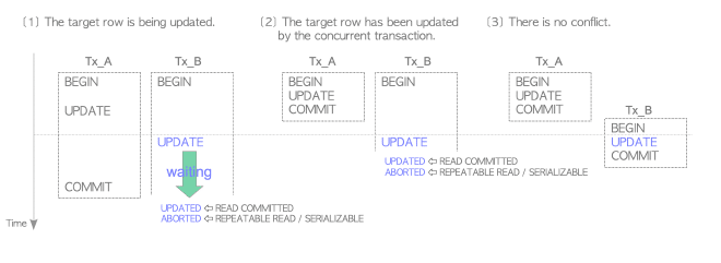
lost update aka ww-conflict: updating of the same rows by concurrent xacts
needs to be prevented in REPEATABLE READ and SERIALIZABLE levels, no need for READ COMMITTED level
pseudocode:
  (1) Get each row for update by this UPDATE command.
  (2) Repeat the following process until the target row is updated (or this transaction is aborted).
  (3) If the target row is being updated, go to step (4); otherwise, go to step (8).
  (4) Wait for the termination of the transaction that updated the target row, because PostgreSQL uses the first-updater-win scheme in SI.
  (5) If the status of the transaction that updated the target row is COMMITTED and the isolation level of this transaction is REPEATABLE READ (or SERIALIZABLE), go to step (6); otherwise, go to step (7).
  (6) Abort this transaction to prevent Lost Updates.
  (7) Go to step (2) and attempt to update the target row in the next round.
  (8) If another concurrent transaction has updated the target row, go to step (9); otherwise, go to step (12).
  (9) If the isolation level of this transaction is READ COMMITTED, go to step (10); otherwise, go to step (11).
  (10) UPDATE the target row, and go to step (1).
  (11) Abort this transaction to prevent Lost Updates.
  (12) UPDATE the target row, and go to step (1), because the target row is not yet modified or has been updated by a terminated transaction (i.e., there is no ww-conflict).
within a while loop, the 3 blocks for the different cases:
when an index page is read (e.g. during any index scan, for both Index-only scans and ordinary index scans)
lock levels and lock aggregation
SIREAD locks may work at 3 levels: tuple, page, relation
so, these locks can be aggregated to save space (e.g. if SIREAD locks created for all tuples within a single page, then the individual-tuple level locks are released and a page-level SIREAD lock is used instead)
when using seqscan, pg creates a relation-level SIREAD lock from the beginning, regardless of indexes or WHERE clauses
this can be a source of false-positive detections of serialization anomalies
rw-conflicts
rw-conflicts can be represented as a triplet e.g. {r=100, w=101, SIREADLOCK={obj=Tuple_1}}— the obj being the object associated with the SIREAD lock
any anomalies from the guarding functions for overlaps, if they detect any anomalies then only the first-committed xact is committed and the other xacts are aborted by the first-committer-wins scheme. the guarding functions:
the space for txnids is fixed and circular and so there’s a wraparound problem that is possible to happen
Figure 11: example of how wraparound can happen
Freeze Processing: solution to wraparound problem #
using FREEZE process to create frozen txid: i.e. a special reserved txid (value 2) which is considered to ALWAYS be older than all other txids
so frozen txid is always inactive and visible to all xacts
VACUUM invokes FREEZE: scans table files and rewrites the t_xmin of tuples to frozen txid (2) if the t_xmin value is older than the current_txid - vacuum_freeze_min_age
       // Phase 1: initializing

(1)    FOR each table
(2)      Acquire a ShareUpdateExclusiveLock lock for the target table

         /* The first block */

         // Phase 2: Scan Heap
(3)      Scan all pages to get all dead tuples, and freeze old tuples if necessary
         // Phase 3: Vacuuming Indexes
(4)      Remove the index tuples that point to the respective dead tuples if exists

         /* The second block */

         // Phase 4: Vacuuming Heap
(5)      FOR each page of the table
(6)         Remove the dead tuples, and Reallocate the live tuples in the page
(7)         Update FSM and VM
         END FOR

         /* The third block */

         // Phase 5: Cleaning up indexes
(8)      Clean up indexes
         // Phase 6: Truncating heap
(9)      Truncate the last page if possible
(10)     Update both the statistics and system catalogs of the target table

         Release the ShareUpdateExclusiveLock lock
      END FOR

      /* Post-processing */

      // Phase 7: Final Cleaning
(11)  Update statistics and system catalogs
(12)  Remove both unnecessary files and pages of the clog if possible
Code Snippet 3:
vacuum phases
some observations:
it’s always index first then the heap
there’s bookkeeping to update:
at the end of phase 6, before releasing the ShareUpdateExclusiveLock
in the final cleaning (phase 7)
ShareUpdateExclusiveLock for the table allows concurrent reads from other transactions
there’s a truncation step for the last page if it’s empty (no tuples)
PARALLEL: if set, and multiple indexes exist, then the index vacuuming and the index cleanup phases are processed in parallel. This parallel feature doesn’t apply to autovacuum.
below is desc of 3 + 1 blocks to the pseudocode
uses a ring buffer, that’s why processed pages are not cached in the shared buffers
first block
for freeze-processing and removing index tuples pointing to dead tuples (vacuuming indexes)
uses maintenance_work_mem (local memory) to store list of dead tuples
if there’s not enough space within local memory, then proceeds to the next steps and returns to this step later (dispatches initial tranche)
second block
works on a page-by-page basis, removes dead tuples and updates FSM + VM
note: unnecessary line pointers are NOT removed, they’re reused in the future.
Removing line pointers would have needed us to update the associated index tuples of the associated indexes
third block
cleanups after index deletion, updating of the statistics and system catalogs for each target table
table-specific VMs that stores the visibility of each page
visibility shows if page contains dead tupels
vacuum processing skips pages without dead tuples — refers to the VM for this
each VM is 1..n 8Kb pages
VM enhancement: allowed freeze processing to be improved in its efficiency also, works by tracking BOTH page visibility and whether all tuples in a page are frozen
2 modes to freeze processing: lazy (typically runs in this mode) vs eager (when specific conditions are satisfied)
also, VACUUM is considered as “lazy” internally
lazy mode: only scan pages that contain dead tuples by using the VM of the target table
eager mode: scan ALL pages regardless of whether they contain dead tuples + updates system catalogs related to freeze processing + removes unnecessary parts of the clog if can
covers the limitations of lazy mode, scans ALL pages, inspects every tuple (for <= v9.5)
compared to the lazy version, the 1st page WON’T get skipped
(> v9.5) VM implementation includes whether ALL tuples in the page are frozen and this helps optimise freeze processing in eager mode — process skips pages that contain ONLY frozen tuples
condition to meet to run freezing in eager mode: pg_database.datfrozenxid < (OldestXmin - vacuum_freeze_table_age)
pg_database.datfrozenxid holds oldest frozen txid for each db
housekeeping updates would include some of these stats too (e.g. pg_class.relfrozenxid)
Note taken on [2026-10-25 Sun 23:40] have to come aback to this section after going through WAL decoding in logical replication
so have to cover:
chapter 9: WAL
chapter 12: Logical Replication
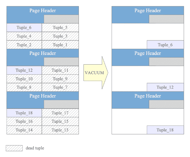
VACUUM can’t reclaim disck space caused by table bloat: when physical size of a table doesn’t decrease even after dead tuples are removed
example case is say there’s 3 pages and after vacuum-ing, each page still has 1 tuple each, so there’s still 3 pages allocated but lots of holes and that’s how there’s table bloat
Figure 13: example of table bloat
generally, issue happens when large volume of dead tuples is generated
solutions:
pre-v18: rebuild the relation fiels and indexes via CLUSTER / VACUUM FULL
both acquire ACCESS EXCLUSIVE locks on the entire table during execution, block ALL operations when rebuilding
disrupts operations during reconstruction, which can be timetaking
REPACK (>= v19) command
both CLUSTER and VACUUM_FULL now use the same implementation too
the lock acquisition can be done CONCURRENTLY, only during file-switching, enabling table reconstruction with higher online availability than before
NOTE: REPACK CONCURRENTLY uses the WAL decoding mechanism that is used in logical replication
this is the REPACK command, not to be confused with a similarly named pg extension (pg_repack)
need to have data durability in face of system failure AND still have performant normal operations
naive approach that is not good enough: flush and sync synchronously from shared memory to storage. problems:
involves whole page
I/O to different locations in storage, can’t have locality optimizations
instead, use a transaction log and track at the tuple-level (small records) appended sequentially
WAL: record the xact changes before writing the corresponding data pages to storage
on terminology: WAL = write-ahead logging (mechanism); “the WAL” / WAL records / WAL segments = the log. XLOG = legacy name for the log, still in source identifiers; user-facing names renamed to wal in PG 10.
all modifications (insertion, deletion, commit actions) are recorded by pg as history data in persistent storage via XLOG records / WAL data
so XLOG records written to in-memoryWAL buffer first
records are uniquely referenced via LSN (Log Sequence Number); it’s an ID + specific location of the record within the log
records flushed to WAL segment file on storage when triggered:
trigger: when a xact finalises (i.e. commits / aborts)
when recovering, it’s key to know when to recover from; it’s the REDO point, the location of the XLOG record written at the moment the latest checkpoint started
recovery and checkpoint processes are tightly related
checkpointer does check-pointing periodically
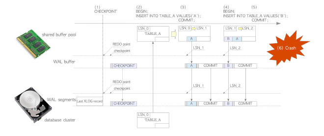
an example
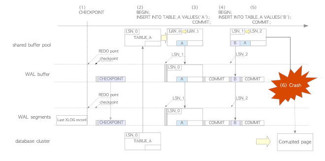
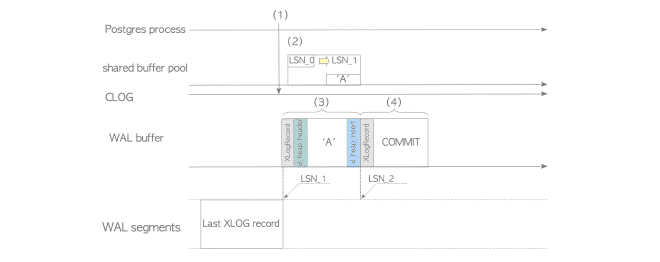
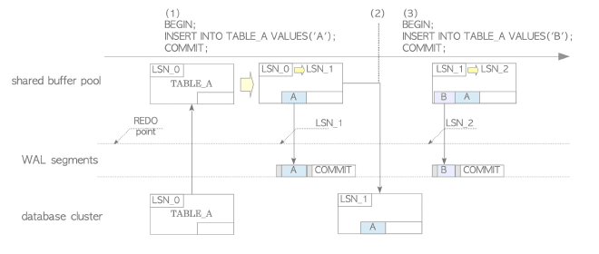
Figure 14: insertion operations with WAL
elaboration:
@ start of a checkpoint, checkpointer writes a checkpoint record (contains latest REDO point) to WAL segment
on first insertion, pg loads the table page into shared buffer pool then inserts a tuple into it and then writes an XLOG record of that statement into the WAL buffer @ LSN_1. It also updates the pd_lsn page header of TABLE_A from LSN_0 to LSN_1
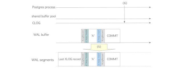
when the xact commits, pg writes commit XLOG record to the WAL buffer, flushes all records from LSN_1 to the WAL segment file
second insert is similar: insert a new tuple, writes an XLOG record @ LSN_2, update table’s LSN to LSN_2
when xact commits, pg flushes XLOG records again
if there’s a system failure, data from shared buffer pool (in-memory data) is lost but modifications persisted in the WAL segment files
so on restarting, pg goes into recovery mode and read-and-replays XLOG records sequentially from REDO point
when doing the replay, there’s some replay rules to check between LSN of XLOG record and the LSN of the page:
if XLOG’s LSN is newer (larger) than page’s LSN then the data portion of the record is inserted into the page and the page’s LSN is updated
if XLOG’s LSN is older (smaller), then the record is skipped
page data on storage may get corrupted if the OS fails when a dirty page is being written; XLOG records can’t be replayed on a corrupted page — need to do a full-page write
here the record needs to be a backup block / full-page image: the XLOG record will contain the entire page during the first modification of the page after a checkpoint
example:
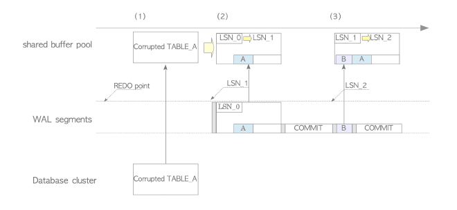
Figure 15: full page writes: example of how page @ storage may be corruptedFigure 16: recovery process
elaboration of how page @ storage may be corrupted:
checkpointer starts checkpoint
first insert triggers creation of backup block since it’s the first modification of the page since the checkpoint
xact commits, wal buffer is flushed
second insert creates a standard XLOG record (and not a backup block) because the page was already modified once since the checkpoint
xact commits
os system failure during checkpointer writing table page to storage – corrupted page on the storage disk
elaboration of how recovery may happen with backup block (ensures data-recovery even if data-write errors occur during crash):
pg reads first XLOG record, loads corrupted page into buffer pool
first record is a BACKUP BLOCK, so the entire page content is overwritten onto corrupted page; regardless of LSN values. The page LSN gets updated to LSN_1 and that’s how the corrupted page gets restored
subsequent non-backup blocks get replayed using the standard LSN rules
doesn’t protect against filesystem / media failure though — have to rely on online backup and replication features to guard against that
sync replication doesn’t eliminate the need for backups
because the failure modes go beyond HW/SW failures, includes Human Error, Software Bugs…
logically, XLOG records get written into a virtual file with 16 Exabytes of space (because it’s an 8-byte address space) — so the transaction log capacity is basically unlimited
pg divides the log into smaller files (WAL segments) ~16Mb each – it’s configurable
the naming follows a particular scheme; WAL segment filename is 24-digit hex number
the default 16Mb WAL segment is divided to 8Kb pages
first page contains a header (XLogLongPageHeaderData (ref)), rest of the pages thereafter have page information defined by the XLogPageHeaderData (ref)
typedefstructXLogRecord{uint32xl_tot_len;/* total len of entire record */TransactionIdxl_xid;/* xact id */XLogRecPtrxl_prev;/* ptr to previous record in log */uint8xl_info;/* flag bits, see below */RmgrIdxl_rmid;/* resource manager for this record *//* 2 bytes of padding here, initialize to zero */pg_crc32cxl_crc;/* CRC for this record *//* XLogRecordBlockHeaders and XLogRecordDataHeader follow, no padding */}XLogRecord;
Code Snippet 4:
self-explanatory struct for what the xlog header looks like(ref)
resource managers: collections of operations for WAL feature (e.g. writing, replaying XLOG records)
how resource managers work:
during the action (e.g. an INSERT statement) then the header variables are set to the resource-manager specific functions
is either a backup block (contains an entire page) or a non-backup block (operation-specific data)
backup block:
has 2 datastructures and 1 data object:
XLogRecord struct (header)
BkpBlock structure: variables that identify page within the db cluster (relfilenode, fork number of relation, block number), also holds starting position and length of the page’s free space
entire page, excluding the free-space (data object)
non-backup block:
layout of data-portion is operation-dependent (<= v9.4)
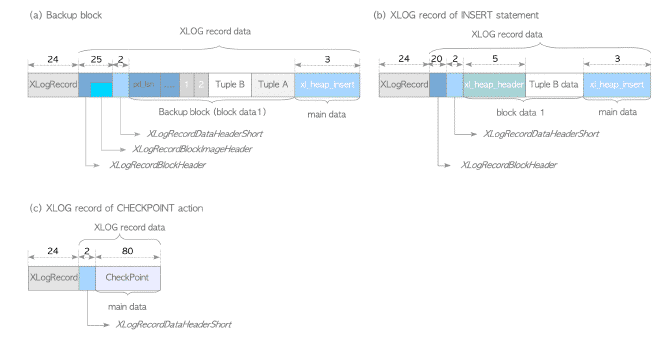
e.g. for INSERT, the XLOG record should have:
XLogRecord (header portion)
xl_heap_insert structure – contains vars to identify the inserted tuple in the database cluster (the relfilenode of the table and the tuple’s TID) and a visibility flag for the tuple.
inserted tuple, less a few bytes
less few bytes because those bytes can be re-constructed
pre 9.5, the problem with XLOG records NOT having a common format is that each RM has to define its own, so it’s hard to maintain the source code and implement new WAL features
so now, there’s a common, structured format that is independent of RMs
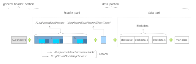
common xlog record format:
Figure 18: common formatFigure 19: Examples of different XLOG records
header part:
header has 0..n XLogRecordBlockHeaders, 0..1 XLogRecordDataHeaderShort / XLogRecordDataHeaderLong — must have at least one of these
if the record is for a FPI (full-page image) then XLogRecordBlockHeader includes XLogRecordBlockImageHeader. If compressed, includes XLogRecordBlockCompressHeader.
data part:
0..n block data (corresponds to XLogRecordBlockHeader s) + 0..1 main data (corresponds to XLogRecordDataHeader)
FPI’s can be compressed using LZ compression method, configurable
evaluating compression of wal FPIs:
con: compression is CPU resource-intensive
advantage: reduces I/O cost for writing records
advantage: suppresses consumption of WAL segment files
the standardisation to the data sections are similar in function to the older approaches, just that the structures are changed
this means the separation of structure between backup blocks vs non-backup blocks are similar – read more here
Logical Replication: when wal_level is logical then there’s a change in behaviour:the actual tuple data is explicitly appended to the main data section, even if an FPI is present
needed for logical replication because the walsender can skip the physical FPI and directly decode the tuple info stored in main data
so, pg achieves an efficient decoding process independent of the physical page layout.
this is important to ensure performance is high and throughput, even during checkpoint spikes surge in WAL volume because of frequent FPI generation right after a checkpoint.
new format for XLOG is optimised for parser efficiency even if it’s more complex and less humanly readable
exec_simple_query() @postgres.c
(1) ExtendCLOG() @clog.c /* Write the state of this transaction
* "IN_PROGRESS" to the CLOG.
*/
(2) heap_insert()@heapam.c /* Insert a tuple, creates a XLOG record,
* and invoke the function XLogInsert.
*/
(3) XLogInsert() @xloginsert.c (9.4 or earlier, xlog.c)
/* Write the XLOG record of the inserted tuple
* to the WAL buffer, and update page's pd_lsn.
*/
(4) finish_xact_command() @postgres.c /* Invoke commit action.*/
XLogInsert() @xloginsert.c (9.4 or earlier, xlog.c)
/* Write a XLOG record of this commit action
* to the WAL buffer.
*/
(5) XLogWrite() @xloginsert.c (9.4 or earlier, xlog.c)
/* Write and flush all XLOG records on
* the WAL buffer to WAL segment.
*/
(6) TransactionIdCommitTree() @transam.c /* Change the state of this transaction
* from "IN_PROGRESS" to "COMMITTED"
* on the CLOG.
*/
Code Snippet 5:
invocation of exec_simple_query() and link to WAL records
Figure 20: Write-sequence of XLOG records (part 1)Figure 21: Write-sequence of XLOG records (part 2)
triggers for writing of XLOG records to the WAL segments:
trigger: a running xact commits / abborts
trigger: WAL buffer fills up (size depends on wal_buffers param)
trigger: WAL writer writes periodically
DML (data-manipulation language) ops generate XLOG records for sure
some non-DML operations can also create XLOG records:
commit action: XLOG record containing the id of the committed xact
checkpoint action: general information about the checkpoint written via an XLOG record
some special cases for select statements:
SELECT FOR UPDATE which generates XLOG records fro all target tuple locks (row share lock)
HOT operations, system writes XLOG records of tuple deletion and page defrag to WAL buffer
bg proc, periodically checks WAL buffer, writes all unwritten XLOG records to WAL segments — avoids bursts of XLOG writing, which may become a bottleneck if large amount of data is written at once
enabled by default, can’t be disabled
wal_writer_delay is the check-interval config, can be changed; defaults to 200ms
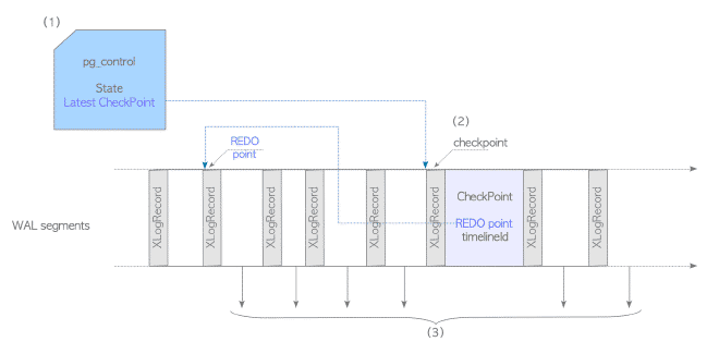
@ start of the recovery proc, the pg_control file is read and its details describe the recovery process from that point
process
Figure 23: details of the recovery process
elaboration:
@ startup of pg instance, pg reads all items within pg_control
if state is ‘in production’ – enters recovery mode (abnormal shutdown) else normal startup mode
read latest checkpoint record from correct WAL segment file using location within the pg_control file, then retrieve the REDO point from the checkpoint record
rmgrs then read-and-replay XLOG records sequentially from REDO point to end of latest WAL segment
if XLOG record is backup block, then the rmgr overwrites the table pages regardless of its LSN, else for non-backup XLOG records, it’s just a replay as long as record’s LSN > pd_lsn of the corresponding page (ref)
the reason why the LSN of a non-backup block and the pd_lsn of the corresponding page needs to be compared, see example:
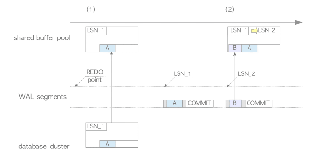
Figure 24: insertion operations during bg writer working (wal buffer omitted for brevity)
pg inserts tuple, writes XLOG @ LSN_1
checkpointer proc writes the table page to storage; page’s pd_lsn is LSN_1
pg inserts new tuple into table and writes XLOG @ LSN_2, modded page yet to be written to storage
if shutdown happens in immediate mode then when it restarts, recovery gets triggerred
Figure 25: db recovery for example
pg loads first XLOG record, and the table page. The record is NOT replayed because the record’s LSN (LSN_1) is not more than page’s LSN (LSN_1) => no need replay
pg replays second XLOG record because its LSN (LSN_2) is more than the current pd_lsn of the table page (LSN_1)
db cluster can become inconsistent if replay order of non-backup blocks is incorrect / extra replays because redo operation is not idempotent
redo operation for backup blocks is idempotent, can be replayed extra times regardless of their LSN
AI usage disclosureClaude Sonnet 5.5 · Primer for Recovery Strategy
This section’s content was AI-generated.
There are several, and they differ mainly in which of two problems they solve and how.
The framing question
After a crash, two things can be wrong with the data files:
Uncommitted changes may be on disk. The buffer manager evicted a dirty page before its transaction committed. Fixing this needs undo.
Committed changes may be missing. The page was still dirty in memory when the crash hit. Fixing this needs redo.
Which problems you can have depends on two buffer-manager policies:
Steal: dirty pages of uncommitted transactions may be written to disk. This is good for memory pressure but creates problem 1.
Force: all of a transaction’s dirty pages must be flushed at commit. This avoids problem 2 but makes commit slow, with random I/O on the critical path.
Every recovery scheme is a choice on this grid:
Policy
Needs undo?
Needs redo?
Example
No-steal + force
no
no
Shadow paging / copy-on-write
Steal + force
yes
no
Undo-only logging
No-steal + no-force
no
yes
Redo-only logging, in-memory DBs
Steal + no-force
yes
yes
ARIES (DB2, SQL Server, InnoDB)
The patterns
1. Shadow paging / copy-on-write (no log). Never overwrite pages in place. Write new versions elsewhere and commit by atomically swapping a root pointer. Recovery is trivial, because you just use whichever root is the last committed one. LMDB, BoltDB, and filesystems like ZFS and btrfs work this way. The costs are random writes, write amplification (you copy the whole path to the root), fragmentation, and difficulty supporting concurrent writers.
2. Undo-only logging. Log the old value before overwriting, and flush the data pages before commit. Recovery rolls back the uncommitted transactions. It’s simple, but forcing pages at commit is expensive, so it’s mostly of historical and teaching interest.
3. Redo-only logging. Never let uncommitted changes reach disk, and log the new values. Recovery replays committed work. The weakness is that a large transaction must fit in memory. This suits in-memory systems well, such as Redis AOF or VoltDB’s command log plus snapshots.
4. Undo/redo logging (ARIES). This is the general solution: steal and no-force give the best runtime performance, and the log pays for it at recovery time. ARIES recovery has three phases:
Analysis: find which transactions were active and which pages were dirty.
Redo: repeat history, replaying everything, including work from transactions that will later be rolled back.
Undo: roll back the losers, writing compensation log records (CLRs) so a crash during undo is also recoverable.
5. Logical or command logging. Log the operation (“run this transaction with these parameters”) rather than the page changes. It’s very compact, but it only works if replay is deterministic, and it needs a consistent snapshot as the starting point. VoltDB does this. It also isn’t idempotent at the page level, so you can’t do the page-LSN trick.
6. The log is the data. LSM trees (WAL plus memtable plus immutable sorted files) and log-structured designs blur the line between log and storage. Aurora takes it further with “the log is the database”: storage nodes materialize pages from the log. Consensus systems (Raft) are similar, recovering by replaying a replicated log from the last snapshot.
Where PG sits
PG is steal + no-force, but it has only a redo phase. There’s no undo phase and no CLRs. This ties back to your earlier visibility question: because MVCC leaves old tuple versions in the heap, rolling back is nearly free. An aborted transaction’s tuples are simply invisible, since clog says ABORTED, and VACUUM cleans them up later. Undo is effectively folded into the visibility rules.
Compare this with InnoDB or Oracle, which keep old versions in a separate undo log or segment. They need that undo log for MVCC reads, and crash recovery uses it for rollback. The costs trade differently:
PG: recovery is simpler and rollback is instant, but you pay in table bloat and vacuum.
InnoDB/Oracle: tables stay compact, but rollback of a big transaction is slow and undo must be managed.
Your notes on idempotency
This is the central design point of redo logging. Replay must be safe to repeat, because you can crash during recovery. There are two ways to get there:
Physical records (backup blocks / full-page images) are naturally idempotent: overwriting a page with a given image twice gives the same result. This is also why PG uses them to protect against torn pages.
Physiological records (physical to a page, logical within it, like “insert tuple at offset 3”) aren’t idempotent. The pd_lsn comparison makes them so, by stamping each page with the last record applied. That turns “apply this change” into “apply this change at most once.”
Pure logical logging has neither mechanism, which is why it needs snapshot-plus-deterministic-replay instead.
The takeaway
Ask what’s allowed to be wrong on disk after a crash, then decide whether to prevent it (force, no-steal, shadow paging) or repair it (undo, redo). Preventing costs runtime performance. Repairing costs log volume and recovery complexity. Most production relational systems repair, because fast commits matter more than fast recovery.
If you want a next step, ARIES’s repeat-history principle and how it differs from PG’s approach would pair well with your WAL notes. The original paper (Mohan et al., 1992) is the canonical reference.
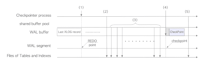
@ start of checkpoint proc, pg estimates, preps the number of WAL segment files needed for the next checkpoint cycle
estimation is based on WAL consumption and previous checkpoint cycles (historical)
counting of WAL segment files is from segment containig the REDO point; has to be between min_wal_size (~80Mb) and max_wal_size (defaults to 1Gb, 64 files)
if total size of the WAL segment files goes beyond it’s allowed bounds, then a checkpoint starts
to minimize system downtime, there was a need for replication even if PITR enabled rapid db restoration after a failure
til 2008, this was contrib middleware (e.g. pgpool-II) so users had to rely on external systems
streaming replication prototype did well (high perf, low WAL processing, low transfer overhead) and so was good enough to be brought into core — see email thread on that here
Streaming Replication in pg uses a single-primary-multiple-standbys architecture
primary server continuously sends WAL data to the standby servers, which immediately replay the received data — so the proc relies on log-shipping (a general replication technique)
cooperation between 3 types of procs in streaming replication:
walsender: proc on primary server
walreceiver: proc on standby server, does the replaying
startup: proc on standby server that starts the walreceiver proc
sequence of streaming replication
Figure 26: SR startup sequence diagram
some notes:
4: walreceiver is the initiator for the TCP connection
5: walsender proc is started to establish the TCP connection between sender and receiver
6: handshaking: walreceiver sends the latest LSN of the standby’s db cluster
7: catch-up phase: if standby’s LSN is less than primary’s latest LSN then walsender sends WAL data for the diff region; it’s the WAL segments from the directory; standby replays the received WAL data
walsender has a states w.r.t working phase of the connected walreceiver / application:
startup: from start to the end of handshaking
catchup: during the catchup phase
streaming: while the replication is working
backup: while sending the files of the whole db cluster for backup tools (e.g. pg_basebackup)
if the standby server restarts after a LONG time (drifts behind too much) then replication slots can prevent the problem of having older WAL segments having already been recycled on the primary
replication slots expand the flexibility of WAL data-sending
2 common failure detection procedures used by streaming replication. Depending on the reason for the failure, detecting it may be immediate or may have a time-lag
immediate failure detection of standby server proc, by primary:
connection drop: primary detects it immediately when on connection drop between walsender, walreceiver
socket error: primary immediately determines failure if low-level network function errors out while accessing walreceiver socket
failure detection of HW and networks:
primary determines network failure if no ack from walreceiver within wal_sender_timeout period
confirming standby’s failure needs up to wal_sender_timeout seconds
not possible to know if no ACK means it’s dark or not so primary has to wait indefinitely
streaming replication lacks a mechanism to auto revert to async mode after a timeout, so all primary server operations get blocked until failure is detected and resolved (including xact commits and subsequent processing of queries)
how to avoid complete blocking of primary operations:
increase availability: multiple standby servers
manual failover to async mode; it doesn’t affect connected clients and the primary server can continue processing xacts and all sessions b/w clients and BE procs are maintained
query conflicts on standbys are well documented within the pg docs on HA here
in streaming replication, standby’s can exec SELECTions independently of primary server
problem: may have conflicts between standby and primary under some situations — possible errors because of replication lags
in the example (ref), the conflict happens because of the WAL data generated by the Access Exclusive Lock which DROP TABLE internally acquires on the primary; which conflicts with the standby’s SELECT command (because WAL-dat includes changes to the data AND also lock information)
typically 3 types of conflicts:
Access Exclusive Locks on primary: conflict with any lock on the standby
dropping dbs or tablespaces
applying vacuum cleanup record from WAL: happens if standby xacts can still see rows being removed or if queries are accessing the affected page
this is troublesome because it’s likely to happen for BOTH VACUUM and autovacuum operations
increasing delays for standby archive and standby streaming reduces conflicts: they allow standby to delay replaying WAL data, so lower likelihood of errors
problem: prevents other backends on the standby from accessing latest data during the delay; also makes the replication not fully synchronous if the delay is bigger
on primary, setting hot_standby_feedback to on avoids vacuum induced conflicts; primary delays deleting data that the standby still needs (based on the standby’s state)
(unimportant) potential / async standby: primary terminates the walsender proc connected to that failed standby, continues all processing
doesn’t affect anything (xact processing) on the primary server
(important) sync standby: associated walsender proc terminated and REPLACED by sync standby with the highest priority potential standby
query processing on primary server to pause until the replacement process for the sync standby is complete
if there’s multiple standby servers in sync mode, then the primary always maintains therequired number of sync standby servers ==> they all must be in a consistent and synchronous state with the primary
struct is ReplicationSlot (ref), shared between both streaming and logical replication
relevant items to streaming replication:
active_pid: pid of walsender proc that manages this slot
ReplicationSlotPersistentData data (saved regularly in pg_replslot dir):
name: of the slot
restart_lsn: oldest LSN that this replication slot may require; checkpointer reads min restart_lsn value across all slots to determine whether WAL segments can be removed
after setting replication slots in shared memory, walsender procs continuously update slots to show current states of the standby servers
primary instance regularly saves detailed info about replication slots to ‘state’ files in pg_replslot dir; on restarting of the primary server, the saved info in pg_replslot is loaded to get back into memory and restore status of its replication slots
Since the introduction of streaming (version 14), logical changes for large transactions may be sent in segments before commit; see Sections 12.1.2 and 12.7. ↩︎
Sequences have been supported since version 19 (2026). ↩︎
TRUNCATE has been supported since version 11 (2018). ↩︎